Eyes, JAPAN
An Introduction to Model Predictive Control (MPC)
Phong
Welcome to my first blog post! I’m kicking things off with a topic I’m truly passionate about: Model Predictive Control (MPC). This was the first framework I ever used in my research, and I believe it’s an essential tool for any control engineer. Let’s dive in and explore how it works.
In the world of control systems, we’re always looking for better ways to steer systems towards a desired behavior. While classic controllers like PID have been workhorses for decades, what happens when our systems are more complex, with multiple constraints and interacting variables? This is where advanced techniques like Model Predictive Control (MPC) come into play.
In this post, we’ll explore the fundamentals of MPC, how it works, and why it’s becoming increasingly popular in a wide range of applications, from autonomous vehicles to chemical plants.
What is Model Predictive Control?
At its core, Model Predictive Control is a control strategy that uses a model of the system to predict its future behavior. Based on these predictions, it calculates the optimal control actions to take.
Let’s break down the name:
- Model: MPC relies on a mathematical model of the system you want to control. This model can be based on physics (e.g., equations of motion) or derived from data. The better the model, the better the control performance.
- Predictive: The “magic” of MPC lies in its ability to look into the future. It uses the model to predict how the system will respond to a sequence of control inputs over a defined time horizon.
- Control: With these predictions, MPC calculates the best possible sequence of future control actions that will minimize a cost function (e.g., minimize error, reduce energy consumption) while satisfying a set of constraints (e.g., actuator limits, safety constraints).
How Does MPC Work? A Step-by-Step Guide
The MPC algorithm works in a receding horizon fashion, which means it repeatedly solves an optimization problem at each time step. Here’s a simplified breakdown of the process:
- Prediction: At the current time, MPC uses the system model to predict the future outputs of the system over a “prediction horizon” for a given sequence of future control inputs.
- Optimization: The controller then finds the optimal sequence of future control inputs by minimizing a predefined cost function. This cost function typically penalizes deviations from the desired setpoint and the magnitude of the control effort. This is where constraints are also taken into account.
- Implementation: Here’s the key part: even though MPC calculates an entire sequence of future control actions, it only implements the first control action in the sequence.
- Repeat: At the next time step, the whole process is repeated. The controller takes a new measurement from the system, updates its prediction, and re-optimizes the control inputs. This constant re-evaluation and correction is why MPC is so robust to disturbances and model inaccuracies.
To visualize this process, let’s look at a typical MPC trajectory:
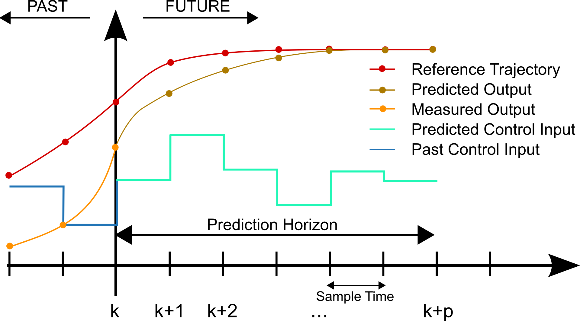

Caption: This chart illustrates the receding horizon principle of MPC. The red line (Desired Setpoint) is our target. The orange line (Output Prediction) shows how MPC predicts the system will respond to the blue line (Optimal Future Control ) calculated over a future horizon. Notice that only the first calculated control action (teal line, Applied Control Input) is actually implemented. At each step, a new prediction and optimization take place, continuously guiding the system towards the setpoint [1].
A Simple Analogy: Driving a Car
Imagine you are driving a car on a winding road. You don’t just look at the piece of road directly in front of your car; you look ahead to anticipate the curves.
- Your mental model of the car (the “Model”) tells you how the car will react to your steering, acceleration, and braking.
- You look ahead (the “Prediction”) to see the upcoming turns.
- You decide on a sequence of steering and speed adjustments (the “Control”) to navigate the turns smoothly and stay within your lane (the “constraints”).
You then start turning the wheel (implementing the first control action). A moment later, you re-evaluate the situation and adjust your plan based on the car’s new position and the road ahead. This is the essence of Model Predictive Control.
Why Use MPC?
MPC offers several advantages over traditional control methods:
- Handles Constraints: MPC can explicitly handle constraints on inputs and outputs, which is crucial for safe and efficient operation of real-world systems.
- Optimal Performance: By optimizing control actions over a future horizon, MPC can achieve better performance compared to reactive controllers.
- Proactive Control: MPC is proactive, not reactive. It anticipates future behavior and takes corrective action in advance.
- Handles Multi-Variable Systems: MPC is well-suited for controlling systems with multiple inputs and multiple outputs (MIMO), where variables are often coupled.
Applications of MPC
The power and versatility of MPC have led to its adoption in a wide array of industries, including:
- Autonomous Driving: For trajectory planning, obstacle avoidance, and adaptive cruise control.
- Chemical and Process Control: To optimize production, improve efficiency, and ensure safety in chemical plants and refineries.
- Robotics: For motion planning and control of robotic arms and mobile robots.
- Energy Management: In smart grids and buildings for optimizing energy consumption.
Reference
[1] MathWorks. (n.d.). What is model predictive control (MPC)? Retrieved October 22, 2025, from https://www.mathworks.com/help/mpc/gs/what-is-mpc.html
- Tweet
-

 2026/02/27
 2026/01/23
 2025/12/12
 2025/12/07
 2025/11/06
 2025/10/31
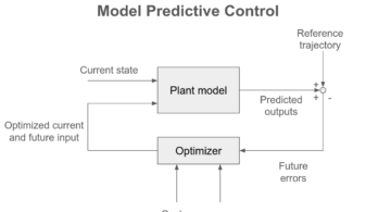 2025/10/24
 2025/10/03